
A little bit of Photoshop® using GNAT for CUDA®
by Olivier Henley –
Most people know about Photoshop®, as it pervades our everyday life when we come across a subway ad, a retouched wedding photoshoot, a set of house staging photos, or the latest profile picture of our favorite Instagram personality.
Today, I want to review some internal mechanisms of a Photoshop-like application to better illustrate an up-and-coming tech, GNAT for CUDA®, developed at AdaCore. To show a real-world example of how one can leverage a heterogeneous architecture model such as CUDA from Ada, I will go over the implementation of an advanced “image transformer” called the bilateral filter:
What is a filter anyway?
Most people do not necessarily know that the term “filter” is a language abuse originating from a subfield of electrical engineering called ‘signal processing’; meaning to remove or filter components out of a signal. It is abuse because our smartphone “photo filters” are not necessarily removing components but behave more like “Transformers” or “Processors” of a signal.
Rest assured that the signal concept is well formalized under mathematical knowledge, meaning we can analyze and process such signals quantitatively and qualitatively. Every year, people present new or better “image transformers” at conferences like ICIP, SIGGRAPH or in specialized publications.
The key takeaway is that a Photoshop “filter” boils down to an algorithm that applies a series of mathematical transformations over the signal components characterizing your image and is still a hot research topic.
And CUDA?
A graphic processing unit (GPU) is a hardware architecture specialized to compute 3D graphics operations. These operations involve a lot of matrices. 3D data generally involves huge sets of linearly independent vectors, which implies that many intermediate results of a final solution can be computed in parallel without affecting one another. Because we know how to build vector-oriented operations directly in silicon, people came up with a hardware architecture inherently more parallel than your typical CPU: a GPU generally presents fewer and simpler silicon operation/block types than a CPU. Specifically organized in parallel silicon stages, these blocks/operations are massively replicated, thus offering the programmer “electrical parallelism” in opposition to “software parallelism,” which can be emulated on a single electrical core. Because the available compute operations are simpler and specialized, they are arranged to optimize calculation throughput; the programmer needs to explicitly adapt its data and operations accordingly. The essence is contained in the term “stream processing”; a GPU architecture is not optimized to handle code branches and sparse data; it’s optimized to “stream” mathematical computations.
For a long time, the programming boilerplate, terminology, and data preparation surrounding the computation over the graphic card were specialized and tightly geared toward 3D graphics. Nevertheless, understanding the computation capability and architecture profile of a GPU, people started to wrap general computation problems stemming from other fields requiring a lot of linear algebra computations (e.g., physics simulation, image processing, AI, big data crunching, etc) over the GPU by “masquerading” the problem within a 3D graphic context (using shaders types, etc.). This is when the expression “general-purpose computing on GPU” or GPGPU came to exist.
With the progression of ubiquitous computing, the need for low latency of highly parallelizable computing exploded in many scientific and engineering disciplines. From there, graphics card designers started to adapt their architecture and API to facilitate “general-purpose” (read “not specifically 3D”) computing on such devices.
CUDA is an NVIDIA™ initiative and one of the most used GPGPU technologies today. NVIDIA is also producing some of the most powerful GPU devices. Taking advantage of such calculation power in Ada is a big deal. Any Ada user having potentially parallelizable problems involving a mix of big data sets and math-intensive calculations with low latency requirements will be legitimately thrilled by this technology.
GNAT for CUDA
We worked hard on GNAT for CUDA’s bindings and programming model to retain Ada’s expressivity while keeping the underlying complexity transparent to the user; a GNAT for CUDA project is uniformly expressed using Ada semantics. Because we are operating over a heterogeneous hardware architecture, your project must build for two targets: the host (CPU) and the device (GPU).
GNAT for CUDA consists primarily of three main parts:
An Ada thick binding to the CUDA libraries. We expose the CUDA API directly in Ada so you can code your project exclusively in Ada.
A small Ada runtime compatible with running on the GPU device. This enables your device object code to exploit the Ada type system, a subset of the standard libraries, etc.
A GNAT frontend to LLVM, able to cross-compile and link device object code. This means you can write Ada code on the host and run it directly on the GPU.
The following is a basic kernel - an entry point in the device code - executed on the GPU, adding two vectors of length Num_Elements. You will find the complete examples in the GNAT for CUDA Git repository. Focus on the core addition C := A + B , as I will detail the critical surrounding technicalities later. Usually, performing this computation with a single thread of execution will take ~O(n) on a CPU. I want to underline the fact that such an addition, through CUDA, will be done in parallel for Num_Elements (given Num_Elements <= CUDA cores) and, therefore, be virtually instantaneous, ~O(1). Now you will have to pay time currency for data transfers A and B from the CPU to the GPU and C from the GPU back to the CPU, synchronization, and some potential sequentiality if you go beyond the CUDA cores thread limits, but this is not pertinent in the face of illustrating the general idea.
procedure Vector_Add (A : Array_Device_Access;
                      B : Array_Device_Access;
                      C : Array_Device_Access) is
...
  begin
     if I < A'Length then
        C (C'First + I) := A (A'First + I) + B (B'First + I);
     end if;
  end Vector_Add;
end Kernel;
Here the parallel computation is made possible by the use of the index ‘I’: it addresses which distinguished ‘silicon unit’ of the CUDA streaming processors will perform the addition.
CUDA 101 on Fast Forward
The gist of CUDA uses four structuring concepts: the grid, the block, the thread, and the kernel. A grid is a group of blocks. A block is a group of threads. A thread executes one or more kernels. A kernel is just a procedure, or code, executed on the GPU like Vector_Add.
A typical NVIDIA GPU has many physical streaming multiprocessors (SM), which in turn have many processing blocks (eg. 4), each of them owning shared memory, ALUs (cores), warp schedulers, an instruction buffer, register file, etc.
As a first approximation, the CUDA programming model ties a thread block (group of threads) to execute concurrently (electrically) on one SM. Therefore specifying the grid and block size in conjunction with their indexing for memory access throughout your algorithm can have a significant impact on the overall performance. The device will take care of the details but the scheduling and the memory access made by your kernel are your responsibility. In practice, performance will scale according to the device's physical capabilities but a misuse of the programming model according to the intrinsic architecture of the device can rapidly result in degrading performance.
Making non-coalesced memory access is such an example. If you do not maintain “linear pattern oriented” memory access (eg. neighbor threads access neighbor memory elements, in read or write) by your concurrent threads, you may cause a form of contention and therefore effective throughput can suffer a lot.
In the following example, we specify the number of threads per block and blocks per grid before launching the kernel on the GPU. This compute topology is defined from the host and sent to the CUDA device by passing it to the kernel execution CUDA_Execute:
procedure Main is
  Num_Elements : Integer := 4096;
...
  Threads_Per_Block : Integer := 256;
  Blocks_Per_Grid : Integer :=
                    (Num_Elements + Threads_Per_Block - 1) / Threads_Per_Block;
...
begin
...
   -- Set compute topology to Device and execute kernel
   pragma CUDA_Execute (..., Threads_Per_Block, Blocks_Per_Grid);
...
end Main;
Then, inside a kernel, you can resolve the actual CUDA thread processing it using the grid, block, and thread index runtime information.
The classic case is to use that thread index to dispatch some data subset to the current kernel thread computation. In the Vector_Add example, because we end up creating ‘Num_Elements’ CUDA threads, a given thread ‘I’ will take care of accessing exclusively the data at position ‘I’ to compute C[I] = A[I] + B[I].
package body Kernel is
  procedure Vector_Add
...
     I : Integer := Integer (Block_Dim.X * Block_IDx.X + Thread_IDx.X);
  begin
...
     C (C'First + I) := A (A'First + I) + B (B'First + I);
...
  end Vector_Add;
end Kernel;
Vector_Add ‘streams’ really well as every kernel instance has no interdependence of data and/or results. It also performs coalesced memory access as both the kernel’s hardware position and memory accesses comply with the same topology. An example of non-coalesced access would be if some kernel instances were written in row order and others in column order. You would be right to deduce that this is a single-dimension problem. The CUDA API lets you create and index up to three dimensions (X, Y, Z). Our bilateral filter implementation will make use of two dimensions.
GNAT for CUDA Programming model
Often, type definitions used to compile for the device will be needed for the host compilation too. Here lies a gotcha in the fact that code built for the device is done against a different GNAT runtime and therefore you cannot throw anything you like at it. In other words, do not include something like Ada.Text_IO alongside a type declaration you will need on the device (GPU) because no Ada IO standard interfaces are supported by this GPU runtime. Looking at the GNAT runtime sources shipped with GNAT for CUDA on Github, you can inspect what is available to call. If you need something special, do not hesitate to get in touch to see if it can be squeezed in.
Let's say you go ahead anyway with such careless code: linking for the host (native runtime) will succeed but fail for the device (constrained CUDA runtime), right? This leads to a recommendation: to prepare your project to scale in complexity, we propose that you structure your sources around host code, device code, and common code. This way you can smoothly control the host and device builds using GPRbuild project files capabilities. If unclear, check the example projects shipped with GNAT for CUDA on GitHub.
As mentioned before a CUDA GPU architecture is historically designed for linear algebra operations in a “stream processing” fashion. As your application originates from the host which is expected to provide a handful of complex machine operations, the general orchestration is done there: data preparation, transfer, global synchronization, and state execution are generally the responsibility of the CPU. CUDA’s device-side API primarily deals with inter-CUDA SM and cores operations. This is CUDA-specific knowledge and its usage remains, as is, through the API binding calls.
Any CPU data source needed by the GPU first needs to be copied over to the device memory. Data transfer to the GPU is often argued to be expensive in time currency but if you organize your data properly it can generally be paid once per host-device and device-host transfer. Here is the condensed but complete data and execution round trip for the VectorAdd example:
-- kernel.ads
type Float_Array is array (Integer range <>) of Float;

type Array_Device_Access is access Float_Array
  with Designated_Storage_Model => CUDA.Storage_Models.Model;

-- main.adb
procedure main is
...
  H_A, H_B, H_C : Array_Host_Access;   -- host arrays
  D_A, D_B, D_C : Array_Device_Access; -- device arrays
begin
  H_A := new Float_Array (1 .. Num_Elements);
...
  D_A := new Float_Array'(H_A.all);       -- a device copy
  D_B := new Float_Array'(H_B.all);       -- a device copy
  D_C := new Float_Array (H_C.all'Range); -- a device array of same range

  pragma CUDA_Execute (Vector_Add (D_A, D_B, D_C),
                       Threads_Per_Block,
                       Blocks_Per_Grid);
...
  H_C.all := D_C.all; -- copy back to host
...
end;
First, we create types Float_Array and Array_Device_Access to hold our data, the vectors, respectively on the host and the device. Ada array types cannot be passed directly from host to device - they need to be passed through specific access types associated with the device memory space. This is done by adding the aspect Designated_Storage_Model => CUDA.Storage_Models.Model to the type targeting the device. Behind the scenes, allocation and deallocation are done through CUDA API allocators. Copies between these pointers and host pointers are also instrumented to be able to move device data to the host and back.
Note that this device pointer has to be pool specific, it can not be access all. It conceptually points to a specific pool of data, the device memory. Therefore conversions to/from other pointer types are not allowed to prevent nonsensical operations.
Highly parallelizable, compute-intensive problem
At runtime of an application like Photoshop, regardless of the image serialization file format (like .jpeg, .png, or .psd) we usually handle in memory image data as raw 2D arrays of red, green, and blue information. We often call those buffers, image buffers, bitmap, pixmap, etc.
Most simple numeric filters are adaptations of mathematical analytic solutions in the discrete domain, eg. numeric convolutions. Others, more complex, are often described as nonlinear because they often combine different mathematical operators breaking output proportionality. Nonlinear filters, algorithmic or even heuristic in nature are generally complex to compute but often provide more powerful results.
You may be wondering why I am talking about all this. Usually, image processing is computationally very costly and, to make matters worse, sometimes tied to soft real-time requirements updates, eg. continuous image segmentation in robotics. Image buffers contain a lot of data (a standard raw HD image frame is 1920x1080x24bit ~ 6MB), filter computations generally need to visit all of it, and operators apply on at least two dimensions. This is where a single instruction, multiple threads (SIMT) computation platform like CUDA becomes handy, sometimes even a necessity. The opportunity to leverage such compute capabilities within a battle-tested engineering-grade programming ecosystem like GNAT offers a productive and holistic experience.
The bilateral filter (Photoshop's Surface Blur)
This is a very interesting classic nonlinear denoising filter as it removes salt and pepper noise while adaptively preserving important image details. As you will see it is also compute-intensive in both data and code. First, let’s detail the implementation problem we are facing using its mathematical definition:

| \(I\) | The image |
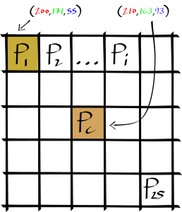
| \(P_c\) | The center pixel of a kernel window |
| \(W_{sc}\) | The spatial and color normalization factor |
| \(\Omega\) | The kernel window |
| \(g_s\) | The spatial Gaussian |
| \(dist_s\) | The spatial distance |
| \(g_c\) | The color Gaussian |
| \(dist_c\) | The color distance |
For every pixel \(P_c\) of the image \(I\), we execute some code, a CUDA kernel, that will transform it: \(I^{filtered}(P_c)\). The kernel \(\Omega\) is centered over \(P_c\) and is parameterized as an \(x\) by \(y\) window of pixel neighbors. Here is a 5 by 5 kernel centered at a given \(P_c\):
Conceptually, this filter necessitates three main computations over the kernel window; a spatial Gaussian blur, a color distance Gaussian and an intensity normalization factor.
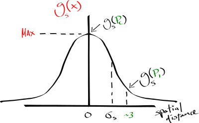
1. Spatial Gaussian blur: \(g_s\). This operation takes care of removing the salt and pepper image noise. Evaluated as a bell shape kernel, the further a neighbor pixel is from the center pixel of interest \(P_c\) the less it is weighted in the summation of the filtered, transformed pixel value. In other words, this operation injects the neighbor's color information, following a Gaussian function of the neighbor's distance from the center, into the filtered pixel of interest. Exposed as a filter control parameter, modifying the standard deviation spatial of the Gaussian, the “fatness” of the function, effectively changes the width of the kernel window.
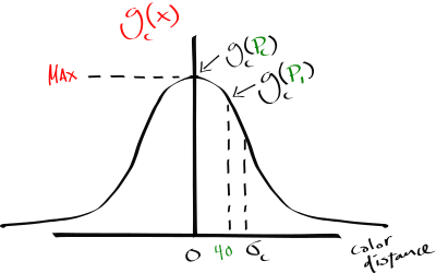
2. Color Gaussian: \(g_c\). Because 1) is a classic blur that deteriorates every picture's detail, and the image’s high frequencies, the following operation is multiplied to modify the blur weight as a function of the given pixel’s color distance from \(P_c\). In other words, “similar” color neighbors will have adaptively heavier participation in the blur, thus statistically biasing the blur on \(P_c\) to retain important details from the kernel’s window perspective.
3. A normalization factor. Because 1) multiplied by 2) are modifying the neighbor pixel's influence non-uniformly over the summation, we need to make sure the initial pixel intensity is recovered; else you would get an over or under-exposed resulting image.

Before moving on, a note is of order. As you can see, even though a Gaussian is a continuous function we only iterate over a finite kernel size; this is an approximation due to porting the function to the discrete domain a Turing machine requires. The "classic" implementation uses a Gaussian but many other filtering profiles can be used, also potentially much friendlier to compute in the discrete domain. Also, we omitted the mathematical definition of \(dist_s\) and \(dist_c\). This is how most papers present the problem, omitting those definitions, as there exist different ways to measure the distance metrics. In our implementation, we use the Euclidean distance, \(dist_n = \sqrt{\sum_{i=1}^{n} (p_{i} - q_{i})^2}\) for both the spatial and color distance as it works quite well for our demonstration needs.
Implementation
For this filter implementation, we first fetch the controlling parameters from the command line using the Generic Command Line Parser (GCLP) by Riccardo Bernardini and then load an input image in the Quite OK Image format (QOI) format using qoi-spark by Fabien Chouteau. We then proceed by filtering the image and finally output the result again in QOI format.
This time we are facing an inherently 2D problem, so let’s create an analogous compute topology. Starting from the previous reasonable assumption of 256 = 16*16 threads per block, we get:
package IC renames Interfaces.C;
package CVT renames CUDA.Vector_Types;
...
Threads_Per_Block : constant CVT.Dim3 := (16, 16, 1);
Block_X : IC.Unsigned := (IC.Unsigned (Width) + Threads_Per_Block.X - 1) /
                          Threads_Per_Block.X;
Block_Y : IC.Unsigned := (IC.Unsigned (Height) + Threads_Per_Block.Y - 1) /
                          Threads_Per_Block.Y;
Blocks_Per_Grid : constant CVT.Dim3 := (Block_X, Block_Y, 1);
Because the data transfer and the execution steps are similar to what was covered in the Vector_Add example we will not detail these here. Feel free to consult the code available at the project repository. By exposing the \(P_c\) index I, J as part of the filter signature we get to support running the bilateral code on both CPU and GPU. Note how we guard the execution of the platform agnostic procedure Bilateral (..., I, J). Because there is no guarantee the data input will be modular to the rounding of the calculated CUDA compute topology we previously determined, you need to guard the kernel execution over irrelevant indices I, J. Here is the GPU path:
package CRA renames CUDA.Runtime_Api;
...
procedure Bilateral_CUDA (...
                          Device_Filtered_Img : G.Image_Device_Access;
                          ...) is
   I : constant Integer := Integer (CRA.Block_Dim.X * CRA.Block_Idx.X +
                                    CRA.Thread_IDx.X);
   J : constant Integer := Integer (CRA.Block_Dim.Y * CRA.Block_IDx.Y +
                                    CRA.Thread_IDx.Y);
begin
   if I in Device_Filtered_Img.all'Range (1) -- guarding index "overflow"
      and then J in Device_Filtered_Img.all'Range (2)
   then
      Bilateral (..., I, J);
   end if;
end;
In the declaration section of the filter we leverage some generics by instantiating a math package for floats as Fmath, we locally define inaccessible helper functions like Compute_Spatial_Gaussian and finally compute the kernel bounds before evaluating the kernel window:
procedure Bilateral (..., I, J) is
   Kernel_Size : constant Integer := Integer (2.0 * Spatial_Stdev * 3.0);
   Half_Size : constant Integer := (Kernel_Size - 1) / 2;
   Spatial_Variance : constant Float := Spatial_Stdev * Spatial_Stdev;
...
   -- Instantiate a math package for floats
   package Fmath is new Ada.Numerics.Generic_Elementary_Functions (Float);
...
   function Compute_Spatial_Gaussian (K : Float) return Float is
   begin
      return (1.0 / (Fmath.Sqrt (2.0 * Ada.Numerics.Pi) * Spatial_Variance)) *
             Fmath.Exp (-0.5 * ((K * K) / Spatial_Variance));
   end;
...
     -- Compute Kernel in X (b)egin, (e)nd
     Xb : constant Integer := I - Half_Size;
     Xe : constant Integer := I + Half_Size;
...
begin
...
end;
The ‘code story’ of the kernel window simply becomes:
procedure Bilateral (..., I, J) is
...
begin
   for X in Xb .. Xe loop -- Loop in X the kernel window centered at I
       for Y in Yb .. Ye loop -- Loop in Y the kernel window centered at J
...
           -- Compute Distances
           Spatial_Dist := Fmath.Sqrt
                           (Distance_square (Float (X - I), Float (Y - J)));
           Rgb_Dist := Fmath.Sqrt
                       (Graphics.Distance_square (Img (I, J), Img (X, Y)));
           -- Compute Gaussians
           Spatial_Gaussian    := Compute_Spatial_Gaussian (Spatial_Dist);
           Color_Dist_Gaussian := Compute_Color_Dist_Gaussian (Rgb_Dist);
           -- Multiply Gaussians
           Sg_Cdg := Spatial_Gaussian * Color_Dist_Gaussian;
           -- Accumulate
           Filtered_Rgb := Filtered_Rgb + (Img (X, Y) * Sg_Cdg);
           -- Track To Normalize Intensity
           Sum_Sg_Cdg := Sum_Sg_Cdg + Sg_Cdg;
...
       end loop;
   end loop;

   if Sum_Sg_Cdg > 0.0 then -- Normalize Intensity
       Filtered_img (I, J) := Graphics."/" (Filtered_Rgb, Sum_Sg_Cdg);
   else
       Filtered_img (I, J) := Img (I, J);
   end if;
end;
Et voila! You get a high-performance, heavily parallelized, bilateral filter, an advanced adaptive nonlinear filter akin to the Photoshop “surface blur” in the Ada programming language leveraging your laptop NVIDIA graphic card.
Note that the kernel here contains loops and conditions. This is perfectly acceptable since we have two accumulators Filtered_Rgb and Sum_Sg_Cdg. Advanced CUDA developers would know that there are even more efficient ways to implement this kind of computation by using a reduction. This last optimization is left to the brave reader.
Results


The top image is the reference (RGB : 1620x1080x24b) and the bottom is our bilateral filtered implementation result using (spatial= 8.0, color= 80.0, RGB : 1620x1080x24bit). Be convinced that we are doing much better than a normal blur. We lose some details but not that much. Actually, we end up with a focal enhanced image that preserves sharp and important features only. Importantly, the big dots of noise, a mix of water splashes, air dust, and image noise, are mostly gone.
Same code, same laptop (CPU: i9-10885H @ 2.40GHz, GPU: NVIDIA RTX 3000 Mobile), excluding the serialization code, the CPU version of the filter took 245.62 seconds while the CUDA version took 0.394 seconds. This represents a ~623x speedup for my particular setup! For this problem, an increase in the kernel window size has a quadratic computational cost on the single-thread CPU version while having a linear cost for the GPU (up to a limit) version as kernel windows are evaluated in parallel. This massive increase in performance can be obtained easily using GNAT for CUDA. With properly organized code as explained before, the adaptation to run on the GPU is almost transparent. We could have multithreaded the CPU version to further our performance analysis but this is left as an exercise for the reader!
I need to emphasize that for didactic purposes I conveniently refrained from doing any optimizations on this demo project to preserve maximum correspondence with the theory; eg. We are computing very precise and "convenient" square roots and some constant Gaussian terms in every kernel instance instead of precomputing them once and for all. It is possible to push the envelope and make new speedup gains but in all moderation, the results are already pretty good!
Final Words
We hope this contextualized presentation of GNAT for CUDA gave you an inspiring overview of the technology and what it can do for you. We think that Ada's verification-centric features like strong typing and rich static analysis are bringing undeniable benefits to GPGPU development. More so, we hope you detected our excitement about bringing this project to fruition and hopefully convinced you to give it a spin for your next compute-intensive project!
https://people.csail.mit.edu/sparis/bf_course/course_notes.pdf
https://github.com/AdaCore/cuda
About Olivier Henley

The author, Olivier Henley, is a UX Engineer at AdaCore. His role is exploring new markets through technical stories. Prior to joining AdaCore, Olivier was a consultant software engineer for Autodesk. Prior to that, Olivier worked on AAA game titles such as For Honor and Rainbow Six Siege in addition to many R&D gaming endeavors at Ubisoft Montreal. Olivier graduated from the Electrical Engineering program at Polytechnique Montreal. He is a co-author of patent US8884949B1, describing the invention of a novel temporal filter implicating NI technology. An Ada advocate, Olivier actively curates GitHub’s Awesome-Ada list