This post is a tale of my introduction to the Ada language with a first project, taking elements from the Raytracing in One Weekend series. Having followed these books in Rust and C++ before, it only made sense to try again in Ada, to understand what the language could bring to a project I’d already explored in depth. All the code used to generate the images in this post is available in this repository.

Raytracing uses the principles of geometrical optics to produce life-accurate renderings of predefined scenes. Most digital rendering techniques are built around rasterization: rendering primitive objects (like triangles) to the screen by converting them to pixel groups directly, and manipulating their position in space and appearance with complex mathematical operations. Raytracing takes a very different approach, by casting millions of light rays into a scene, often hundreds or thousands per pixel, and simulating each light ray’s path until it exits the scene or travels a maximum distance.

For a long time, this approach was completely infeasible for real-time rendering (for instance in a video game, where the software must create 60 images per second, or even more). On modern GPUs, real time rendering has been made possible by greatly reducing the number of light rays used, and using smart smoothing algorithms. This project does not focus on real time rendering however, and instead prioritizes accuracy, even if it means an image can take minutes to render.

In C++, I’d already gone much further than in my first Rust version (although not because of the merits of the language). My first objective in Ada would be to load a 3D model from an external source (I picked the Utah Teapot, a classic in 3D rendering).

Part of what fascinates me about raytracing, and programming in general, is how wonderfully complex behaviours emerge out of simple rules. In “Raytracing in One Weekend”, we go from the simplest structures (3D points and vectors, “rays” made from a starting point and a direction) and very quickly manage to get satisfying images by simulating extremely simple physical rules. So, let’s dive in!

Building 3D geometry primitives

I’d never done any Ada before, so I started with the learn.adacore.com website and the Introduction to Ada course. This was pretty useful as a first knowledge base, as online documentation for the language is sparse, and the Ada Reference Manual is meant for detailed information lookup and not for learning the language.

After playing around with the usual Hello world, I quickly looked up how to structure my program; first with packages and splitting a large program in several files, and then with defining custom types. The first thing I built was a module to do 3D geometry in, using simple structures:

Raytracing techniques follow the laws of geometrical optics, and as such need a lot of vectors and operations on them. It’s a lot of math, so I quickly reached for the operator overloading capabilities of Ada, in order to easily define vector (and point) addition, multiplication and division by a scalar value. From these, it became easy to cleanly define operations like the dot product, cross product, and friends. I was very pleased with the simplicity of defining these operators, and with the strength of the type system that ensured I was never misusing functions or procedures.

I also implemented a small random number generator (RNG) based on Xoroshiro128+. The raytracing process is inherently stochastic (it uses a lot of randomness which is then averaged out to produce a clean image). I did not know the performance characteristics of the standard library random numbers, so I chose to implement one I knew would be very fast. Almost every bounce of a ray needs to produce a new, random direction, so having fast random number generation was a priority. Besides, we don’t need a high randomness quality in the RNG, it’s not like we’re doing cryptography.

Creating objects and images

Geometric primitives aren’t that useful if we cannot see them. The program needs to be able to output an image. Thankfully, I was using the alire package manager, similar in spirit to Rust’s cargo, so I could very easily use an external dependency: the Image_IO crate, with a simple API that allowed me to produce PNG images from pixel arrays. This library, and a JSON parser, were the only two external dependencies of the project, everything else being done by hand.

The alire command line tool (alr) coordinates builds and runs the program, making the development process pleasant. Despite the small size of the Ada open source community, there are quite a few packages available, and alire makes using them a breeze.

To be able to actually show interesting things on the screen, we need a camera to cast rays into the scene, randomly covering every pixel’s surface; but most of all we need objects to actually show onto the screen. I wanted to (at least) have spheres and triangles to show. In Rust and C++, I had used dynamic dispatching, respectively with dyn Trait syntax and virtual function calls, to have different intersection methods on different primitives (spheres, triangles, parallelograms, cylinders…). I tried at first to reproduce this in Ada, but eventually decided against it and used a discriminated type instead.

This basi­cal­ly mir­rors the enum types from rust, sum types from OCaml, and is usu­al­ly called a dis­crim­i­nat­ed union in the C/C++ worlds (although they do not have lan­guage sup­port). Ada has the added ben­e­fit over Rust enums that I can define shared fields for all dis­crim­i­nants, as with the Mat field in this exam­ple. A lit­tle trick I learned is that dis­crim­i­nat­ed types with­out a default val­ue for the dis­crim­i­nant are unsized, mak­ing it nec­es­sary to pro­vide a dis­crim­i­nant val­ue when­ev­er an object is cre­at­ed. In con­trast, adding a default (here with := Sphere) allows cre­at­ing objects with­out spec­i­fy­ing a dis­crim­i­nant val­ue; all such objects have the same size, name­ly the max­i­mum size need­ed for any dis­crim­i­nant. This makes it pos­si­ble to store them in an array, and I would need to do so when build­ing com­plex scenes with a lot of dif­fer­ent objects. This kind of behav­iour is a lit­tle sur­pris­ing as a new­com­er, and hard to dis­cov­er with­out guidance.

Now, for each kind of prim­i­tive, we can use the appro­pri­ate inter­sec­tion func­tion (with anoth­er case block). When cast­ing rays into a scene, the pro­gram needs to check the clos­est object it hits, and then react to that col­li­sion accord­ing­ly. One of the sim­plest shapes to ren­der is the sphere, as express­ing the dis­tance to a sphere is very easy; for a ray with ori­gin O and direc­tion d, and a sphere with cen­ter C and radius r, we just need to solve distance(O+td, C)=r, which can be reduced to a sim­ple qua­drat­ic equa­tion in t.

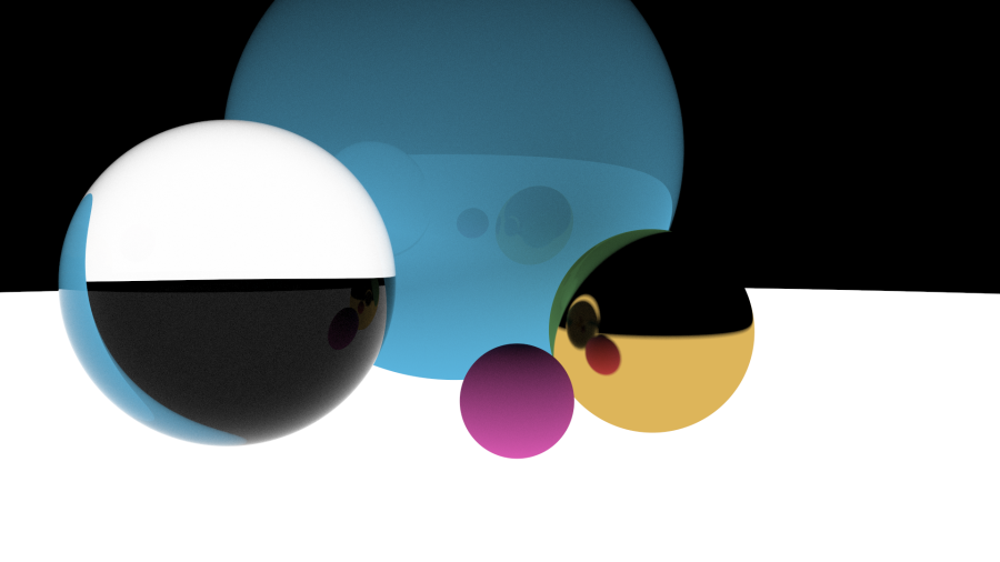
For a first test ren­der, we can just put a cou­ple spheres in an array, and then try to launch a few rays at it; when a ray col­lides with a sphere, we make it bounce back in a ran­dom direc­tion (accord­ing to the sur­face normal).

We cap the bounces to a small fixed lim­it. Ini­tial­ly, the ray is pure white light. When hit­ting a sur­face, we mul­ti­ply it with a fixed col­or (lat­er on, we will add real, con­fig­urable mate­ri­als) and when it doesn’t hit any­thing, we mul­ti­ply it by the ​“sky” color.

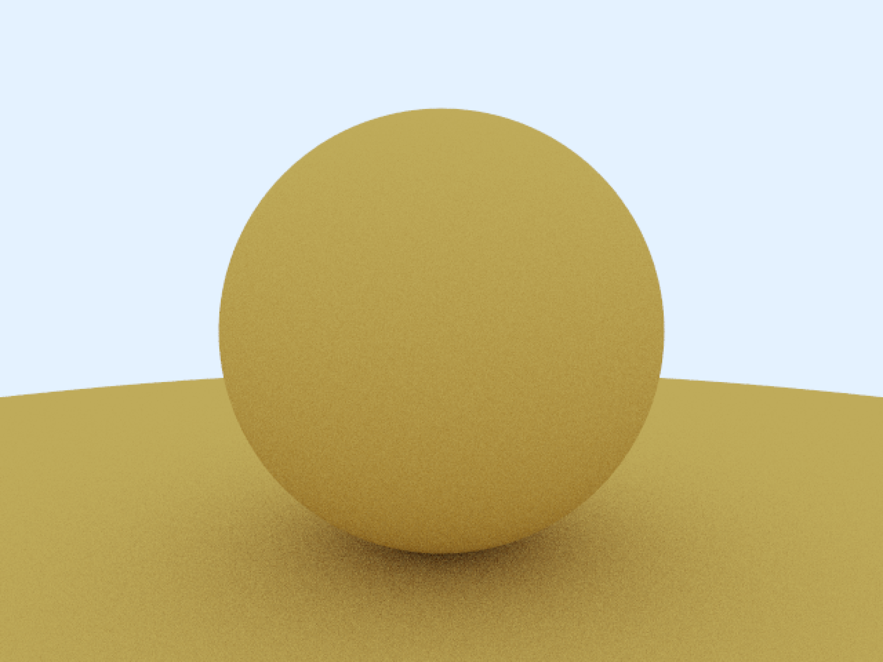
This simulates ambient lighting pretty well already! Since the rays all bounce in random directions, we need to have at least a hundred or so of them per pixel, otherwise the image would be quite noisy:

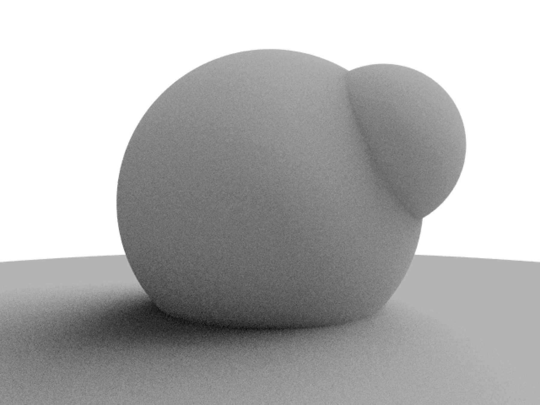
(Additionally, in this picture, the bounces weren’t properly equidistributed in the surface half space, hence the directional shadow, born of a bias bug in the random direction generation).

You may have noticed that the raytracing process operates in reverse compared to real life light rays: instead of going from light source to camera, we go from camera to light source (here, the sky). This is because most rays emitted from the source would never reach the camera; instead, we only trace the rays that reached the camera back to their source. And geometrical optics have that wonderful property that ray paths are independent of the direction of time, meaning a ray from B to A and from A to B take exactly the same path.

Parallelism in Ada

This kind of raytracing is what is called an "embarrassingly parallel” problem. Thousands of rays are launched and never interact with each other, they just get summed up once per pixel and then written to an image grid. We could theoretically have one core running per pixel without any synchronization mechanisms. In practice, we don’t have that many cores, so we don’t really need to parallelise to such an extent. Instead, I chose to parallelise my program on pixel columns.

The Ada language provides a built-in parallelism implementation, called tasking. In a package or a subprogram, one can define tasks, or task types when a task needs to be reused; these are execution units that will run in parallel to the main unit. There are some easy to use synchronization primitives, like entries: a basic communication channel that can synchronize two execution threads.

I used these constructs to build a primitive dynamic thread pool to parallelize the rendering. It needs to be dynamic; when casting rays, there are regions where it will bounce a lot before exiting the scene, regions where there are more objects to check for collisions, and regions where more complex interactions with the materials take more time to compute. In order to avoid starvation in the task pool, we need to be able to send work as needed to tasks that have nothing to do.

The task pool has a coordinator task, and several worker tasks. On startup, the worker tasks send a “ready” notification to the coordinator, which will then send them a work unit (in our case, a pixel column to process). When that work unit is done, the worker task sends a new ready message. I implemented this design as a generic package, allowing it to potentially be reused for other projects.

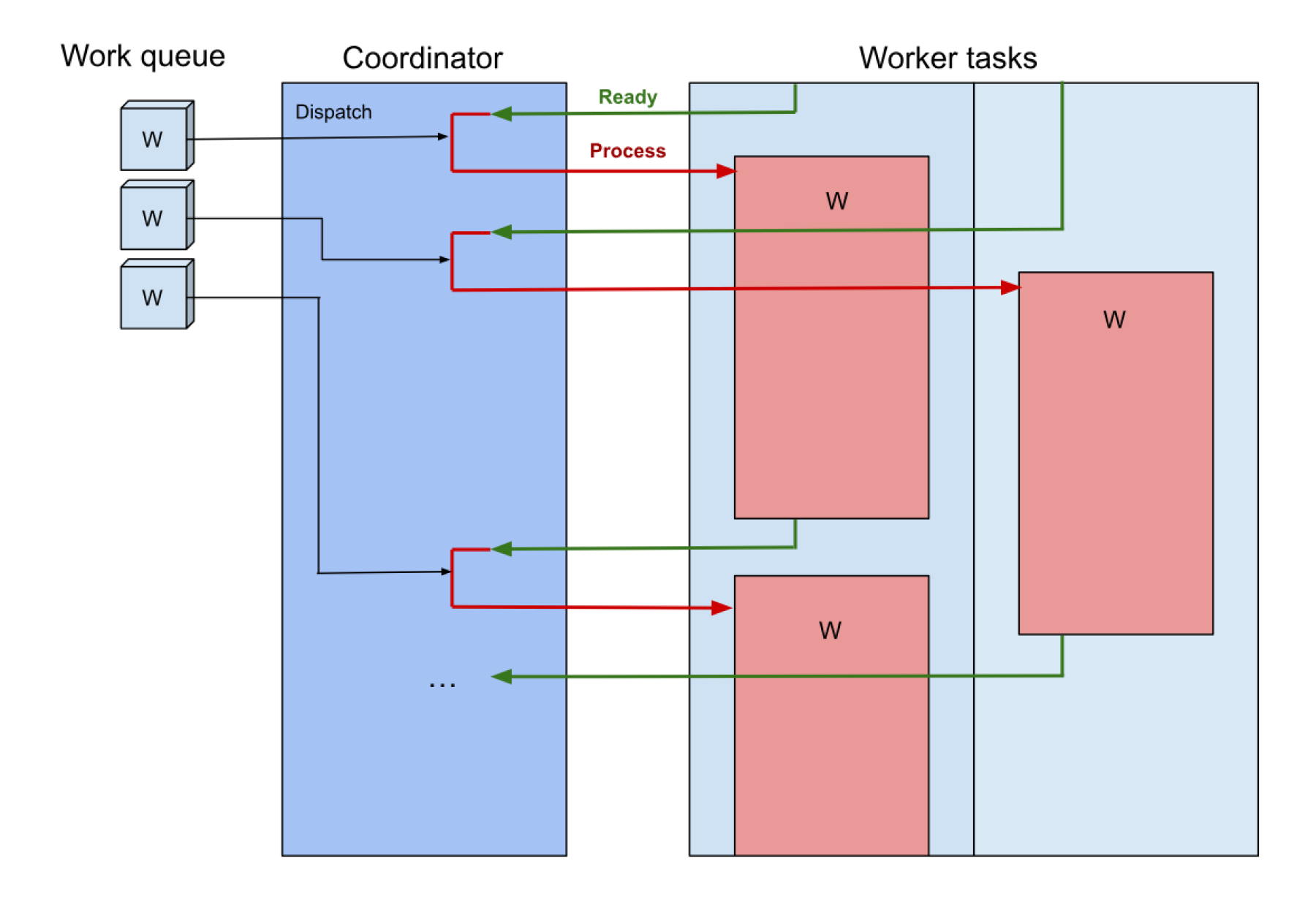
I was really impressed with the built-in parallelism capabilities of Ada; this flexible architecture spans a tiny amount of code. It gave me a near perfect speedup (which is easy to say for such an obviously parallelisable algorithm), and I could generate very high quality images in a matter of minutes (when using a lot of samples per pixel).

Unfortunately, tasking has unwanted side effects in the current implementation. I mentioned earlier that I wasn’t able to use dynamic dispatch and an object oriented style for the scene objects; this is because using those forces me to use managed (“controlled”) objects if I want to be able to store objects in an array. And managed objects, as of 2024, slow down parallel processing considerably, adding lock contention in unwanted places for reasons not entirely clear to me. I was told this issue is being worked on, however.

Complex scenes

When creating scenes, we want to be able to give different looks to different objects. This means controlling how rays bounce off of a material, which color the object has… With the same strategy as earlier with spheres and triangles, we can create a discriminated Material type, which will encode different behaviours when exposed to light.

The first material we have is the one we worked with earlier: a diffuse surface, scattering rays in random directions. This represents an opaque surface with a fixed color, smooth and non-shiny, like a wall. Then, if we decide instead to make the rays bounce in perfect reflection to the incoming rays, we get a metallic, mirror-like surface. If we want to have a glass-like surface, we need to implement refraction (and partial reflection), the geometrical operation that describes how a ray changes angle when entering a transparent medium like water or glass. Finally, if we want to have a material that emits light instead of absorbing it, we can just stop the ray at the object and multiply it by the light color, thanks to the symmetrical properties of geometrical optics mentioned earlier.

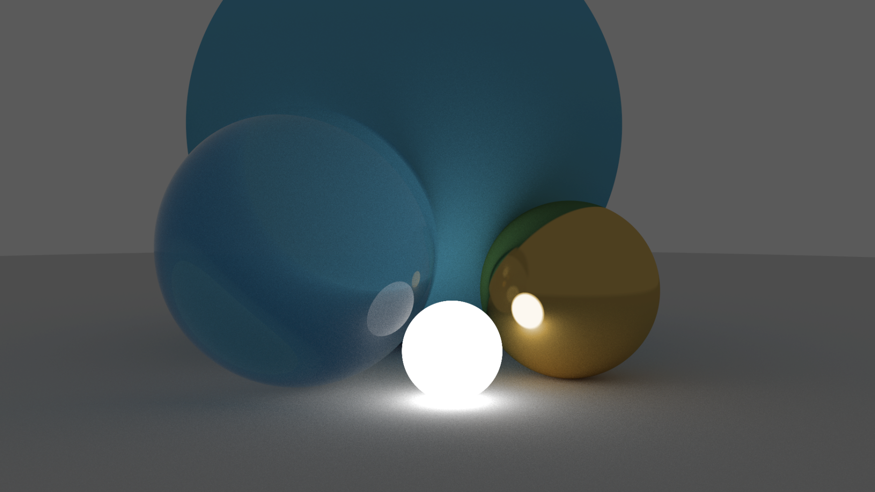
We get different objects with different materials, and so far it looks pretty nice! Until now, we searched for collisions linearly with all objects. And for a scene with 5 spheres, that’s very efficient. But what if we want to render a teapot with 15000 triangles? Going through the list is going to be a bit long. We need a different way to represent our scene, and we need to find a way to avoid computing ALL intersections.

To do that, we’re going to build a binary tree structure; it will allow us to compute only a near logarithmic number of intersections per ray. The scene will be recursively divided along axis-aligned planes, by computing bounding boxes of all our objects and sorting them in two subtrees. We pick our subdivisions according to a heuristic that works very well in practice: we want to minimize the surface area of the subtrees’ bounding boxes. The goal with this tree is to split the scene into nested bounding boxes; when checking for a collision, we will only check for collision with an object if the ray hits every bounding box that contains it. That way, we can (ideally) eliminate half the objects in the scene every time we go down one level in the tree.

Binary tree structures, in most programming languages, would naively be implemented using pointers and allocations for each tree node. In Ada, using pointers is done through access types, but that strategy would be a bit awkward here. Using separate allocations for each tree node would be terrible for cache locality when using our tree structure; and I found that using pointers and manual heap allocations in Ada is somewhat inconvenient, requiring a generic function instanciation to free anything, and making it very hard to use pointers to local data. Instead, we will store our nodes compactly in an array, and the ‘pointers’ will be replaced by indexes into the array. Each node maps to a range of objects in our original object array; we use a quicksort-like procedure to sort the objects so that every object in the same bounding box is in a consecutive range in the array.

This structure takes a while to build with a lot of triangles. When loading an object with 150’000 triangles, my implementation builds and optimises the tree in roughly 30 seconds on my i9-12900H processor But the performance gains for the actual raytracing are well worth it, as instead of doing 150’000 intersection checks we now do on average 50 or so per ray.

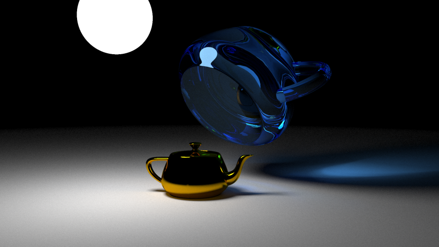
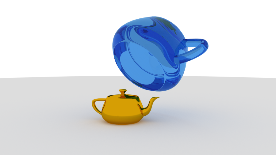
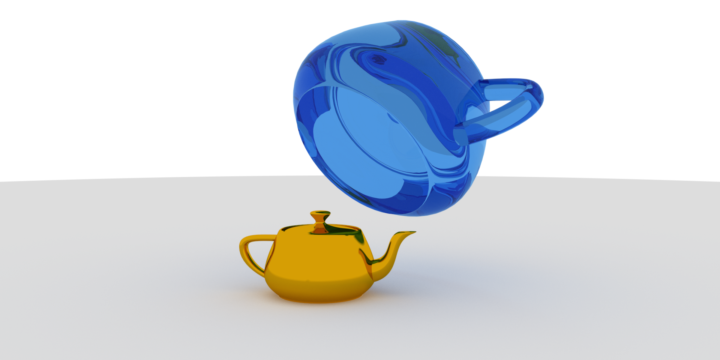
Now, after defining a scene in a JSON file, and parsing the triangle list of our Utah teapot, we can render a very pretty teapot in record times!

Lessons learned

Doing this project in Ada left me with a good impression, with some minor nitpicks. Some things were made very easy, notably all the geometrical computations and definitions. I particularly liked explicit mutability annotations on function and procedure parameters, and the fact that values are encouraged to live on the stack whenever possible, avoiding hidden performance issues and memory unsafety. The language itself makes building strong, reliable abstractions comfortable and natural. Building complex data structures required a bit more effort, parsing a JSON scene file was notably quite unpleasant - but I believe that is mostly because of missing documentation and libraries that don’t get much usage.

What I missed the most, I believe, was having access to a searchable API documentation for the language and its libraries, like in Rust or in C++. It made discovering the capabilities of the standard library a bit awkward, as I could only rely on the AdaCore learning platform and in-person help from people more knowledgeable than I.

But I believe the result to be satisfying enough to call this project a success!