Make with Ada 2020: Ada Robot Car With Neural Network

by Juliana Silva – Nov 05, 2020

Guillermo Perez's project won a finalist prize in the Make with Ada 2019/20 competition. This project was originally posted on Hackster.io here. For those interested in participating in the 2020/21 competition, registration is now open and project submissions will be accepted until Jan 31st 2021, register here.

With this smart robot, we will use a neural network to follow the light and stop when it reaches its goal.

Story

INTRODUCTION

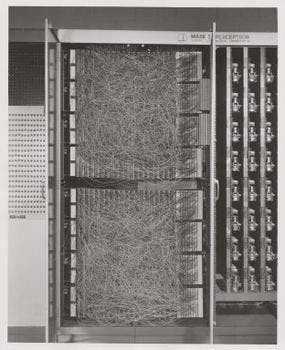
If the robots had to have everything pre-programmed it would be a problem. They simply could not adapt to changes, a "programmer" would have to change the code for the robot to work every time the environment changes. The way to solve it's by allowing the robot to learn and artificial intelligence is a necessary alternative if we want the robots not only to do what we need them to do, but to help us find even a better solution. The perceptron is an algorithm based on the functioning of a neuron. It was first developed in 1957 by Frank Rosenblatt, and here you can check the whole story: https://en.wikipedia.org/wiki/Perceptron

The main goal of this project is to develop a robot car that follows the light emitted by a lamp and through the use of neural networks.

Particular goals:

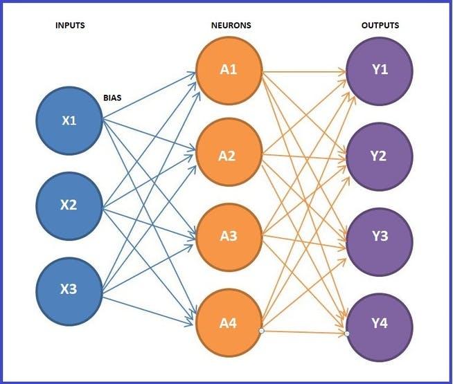
We will use three inputs (including the BIAS), four hidden neurons and four outputs (each one connected to the motors pins). It's important to clarify that some programmers prefer that the robot simultaneously calculate the weights of the neurons and execute the action, and this is the cause a small delay of time. We prefer to calculate the weights using software to avoid these errors.
And also we include an input to stop the robot when it reaches its target from a threshold of light, since many robots continues the move without stopping.

Next, you will find all the information in the following order: Hardware, Neural Network, GPS Project, Assembling the Chassis, Test and Conclusion.

HARDWARE

(Timing: 2 hrs.)

The electrical diagram of this project I show you in the figure below.

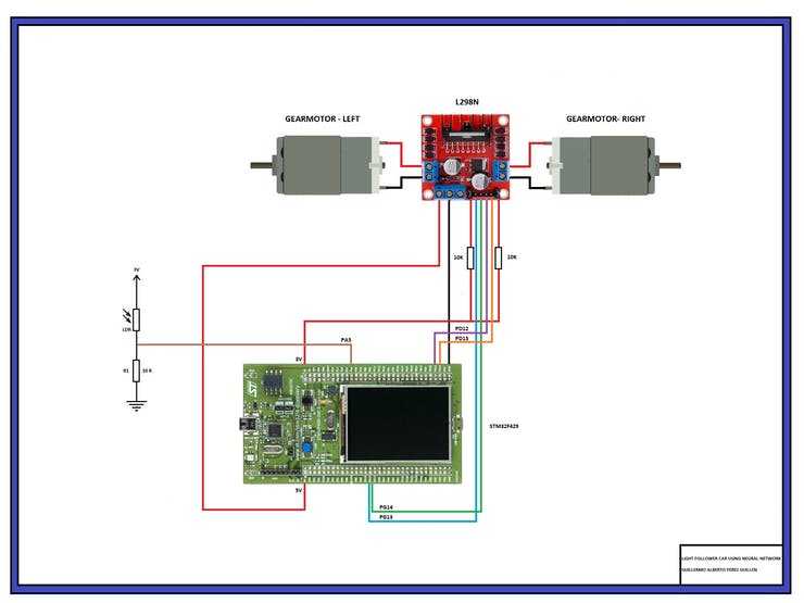
Note: All parts are commercial and easy to get. I recommend that when you assemble the motors do it carefully, since you can connect them in the opposite direction. So make the connections, and then do the tests.

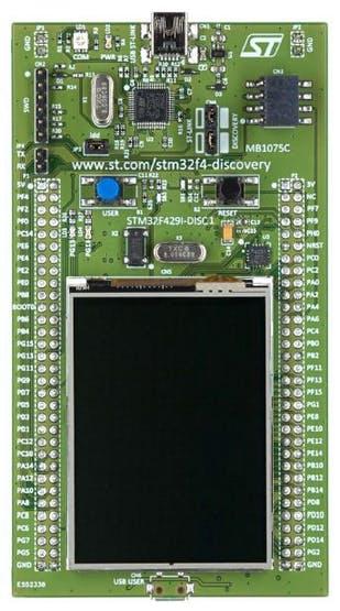
STM32F429I-DISC1

This is the board that I will use for my project, which has many useful tools and a great AdaCore library support.

STM32F429ZIT6 microcontroller featuring 2 Mbytes of Flash memory, 256 Kbytes of RAM in an LQFP144 package
USB functions: Debug port, Virtual COM port, and Mass storage.
Board power supply: through the USB bus or from an external 3 V or 5 V supply voltage
2.4" QVGA TFT LCD
64-Mbit SDRAM
L3GD20, ST-MEMS motion sensor 3-axis digital output gyroscope
Six LEDs: LD1 (red/green) for USB communication, LD2 (red) for 3.3 V power-on, two user LEDs: LD3 (green), LD4 (red) and two USB OTG LEDs: LD5 (green) VBUS and LD6 (red) OC (over-current)
Two push-buttons (user and reset)

Tools, software, and resources on: https://www.st.com/en/evaluation-tools/32f429idiscovery.html

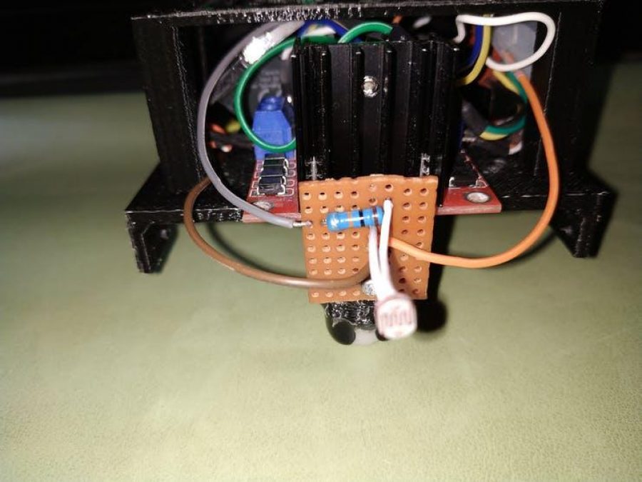
LDR (Light Dependent Resistor)

Two cadmium sulphide(cds) photoconductive cells with spectral responses similar to that of the human eye. The cell resistance falls with increasing light intensity. Applications include smoke detection, automatic lighting control, batch counting and burglar alarm systems.

Datasheet: http://yourduino.com/docs/Photoresistor-5516-datasheet.pdf

NEURAL NETWORK

(Timing: 8 hrs.)

A neural network is a circuit of neurons, or an artificial neural network, composed of artificial neurons or nodes. Thus a neural network is either a biological neural network, made up of real biological neurons, or an artificial neural network, for solving artificial intelligence problems. The connections of the biological neuron are modeled as weights. A positive weight reflects an excitatory connection, while negative values mean inhibitory connections. All inputs are modified by a weight and summed. This activity is referred as a linear combination. Finally, an activation function controls the amplitude of the output. For example, an acceptable range of output is usually between 0 and 1, or it could be −1 and 1. https://en.wikipedia.org/wiki/Neural_network

Bibliographic reference:

The theoretical information you can find on several websites, in my case I support my work with the following publication in Spanish: https://www.aprendemachinelearning.com/crear-una-red-neuronal-en-python-desde-cero/

Here the author shows us the theory, and an example to calculate the weights of a neural network with Python and applied to Arduino board. In my case I will make a brief review of how I use this information to do my project with AdaCore. For example I've modified the codes in Python programming language according to my needs, and I'm the author of the GPS codes.

Lets starts

In our robot, what we want to achieve is that it moves, using a light sensor, in a directed way towards the light. The robot will only have two types of movement: move forward, and rotate to the left. We want the car to learn to move forward when its movement brings it closer to the light, and to turn for a time of 100 milliseconds when it moves away from the light. The reinforcement will be as follows:

If the movement improves the light, with respect to its previous position, then it rewards: move forward
And if the movement results in a less light position, then the movement is penalized for not doing so again: turn to the left

I show you the neural network that I designed with three inputs in the figure below, four neurons and four outputs. We can appreciate all the connections that each one represents the hidden weights that we will calculate later using software.

We want our robot to learn to follow the light with only one light sensor. We are going to build a system that takes two inputs: 1) the received light (a value between 0 to 4095) before the movement, and 2) the received light after the movement. In the figure below we can see the table of values of how our neural network would work.

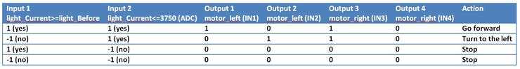
Table of values of inputs, outputs and actions of the neural network.

We can appreciate that there are only four options:

If the current light is greater than or equal to the previous light and we have a light emission of less than 3750, the robot moves forward for 100 milliseconds.
If the current light is less than the previous light and we have a light emission less than or equal to 3750, the robot turns to the left for 100 milliseconds.
In the other two remaining options the robot stops because the light emitted by the lamp is greater than 3750 bits. This means that it's very close to the light.

The Complete code of the "Neural network" with Backpropagation is as follows:

import numpy as np

# We create the class 
class NeuralNetwork:

    def __init__(self, layers, activation='tanh'):
        if activation == 'sigmoid':
            self.activation = sigmoid
            self.activation_prime = sigmoid_derivada
        elif activation == 'tanh':
            self.activation = tanh
            self.activation_prime = tanh_derivada

        # Initialize the weights
        self.weights = []
        self.deltas = []
        # Assign random values to input layer and hidden layer
        for i in range(1, len(layers) - 1):
            r = 2*np.random.random((layers[i-1] + 1, layers[i] + 1)) -1
            self.weights.append(r)
        # Assigned random to output layer
        r = 2*np.random.random( (layers[i] + 1, layers[i+1])) - 1
        self.weights.append(r)

    def fit(self, X, y, learning_rate=0.2, epochs=100000):
        # I add column of ones to the X inputs. With this we add the Bias unit to the input layer
        ones = np.atleast_2d(np.ones(X.shape[0]))
        X = np.concatenate((ones.T, X), axis=1)
        
        for k in range(epochs):
            i = np.random.randint(X.shape[0])
            a = [X[i]]

            for l in range(len(self.weights)):
                    dot_value = np.dot(a[l], self.weights[l])
                    activation = self.activation(dot_value)
                    a.append(activation)
            #Calculate the difference in the output layer and the value obtained
            error = y[i] - a[-1]
            deltas = [error * self.activation_prime(a[-1])]
            
            # We start in the second layer until the last one (A layer before the output one)
            for l in range(len(a) - 2, 0, -1): 
                deltas.append(deltas[-1].dot(self.weights[l].T)*self.activation_prime(a[l]))
            self.deltas.append(deltas)

            # Reverse
            deltas.reverse()

            # Backpropagation
            # 1. Multiply the output delta with the input activations to obtain the weight gradient.             
            # 2. Updated the weight by subtracting a percentage of the gradient
            for i in range(len(self.weights)):
                layer = np.atleast_2d(a[i])
                delta = np.atleast_2d(deltas[i])
                self.weights[i] += learning_rate * layer.T.dot(delta)

            if k % 10000 == 0: print('epochs:', k)

    def predict(self, x): 
        ones = np.atleast_2d(np.ones(x.shape[0]))
        a = np.concatenate((np.ones(1).T, np.array(x)), axis=0)
        for l in range(0, len(self.weights)):
            a = self.activation(np.dot(a, self.weights[l]))
        return a

    def print_weights(self):
        print("LIST OF CONNECTION WEIGHTS")
        for i in range(len(self.weights)):
            print(self.weights[i])

    def get_weights(self):
        return self.weights
    
    def get_deltas(self):
        return self.deltas

# When creating the network, we can choose between using the sigmoid or tanh function
def sigmoid(x):
    return 1.0/(1.0 + np.exp(-x))

def sigmoid_derivada(x):
    return sigmoid(x)*(1.0-sigmoid(x))

def tanh(x):
    return np.tanh(x)

def tanh_derivada(x):
    return 1.0 - x**2

########## CAR NETWORK

nn = NeuralNetwork([2,2,4],activation ='tanh') # no incluir la bias aqui porque si la esta en los calculos

X = np.array([[1,1],   # light_Current >= light_Before & light_Current <= 3750
              [-1,1],   # light_Current < light_Before & light_Current <= 3750
              [1,-1],   # light_Current >= light_Before & light_Current > 3750
              [-1,-1],   # light_Current < light_Before & light_Current > 3750
             ])
# the outputs correspond to starting (or not) the motors
y = np.array([[1,0,1,0], # go forward 
              [0,1,1,0], # turn to the left
              [0,0,0,0], # stop
              [0,0,0,0], # stop
             ])
nn.fit(X, y, learning_rate=0.03,epochs=15001)
 
def valNN(x):
    return (int)(abs(round(x)))
 
index=0
for e in X:
    prediccion = nn.predict(e)
    print("X:",e,"expected:",y[index],"obtained:", valNN(prediccion[0]),valNN(prediccion[1]),valNN(prediccion[2]),valNN(prediccion[3]))
    index=index+1

You can run this code with Python 3.7.3, or with Jupiter Notebook, and the result is as follows:

Expected and obtained values with this code

With 15 thousand periods it was enough to get minimal errors. We have to add the following code to see the cost graphic:

########## WE GRAPH THE COST FUNCTION
    
import matplotlib.pyplot as plt

deltas = nn.get_deltas()
valores=[]
index=0
for arreglo in deltas:
    valores.append(arreglo[1][0] + arreglo[1][1])
    index=index+1

plt.plot(range(len(valores)), valores, color='b')
plt.ylim([0, 1])
plt.ylabel('Cost')
plt.xlabel('Epochs')
plt.tight_layout()
plt.show()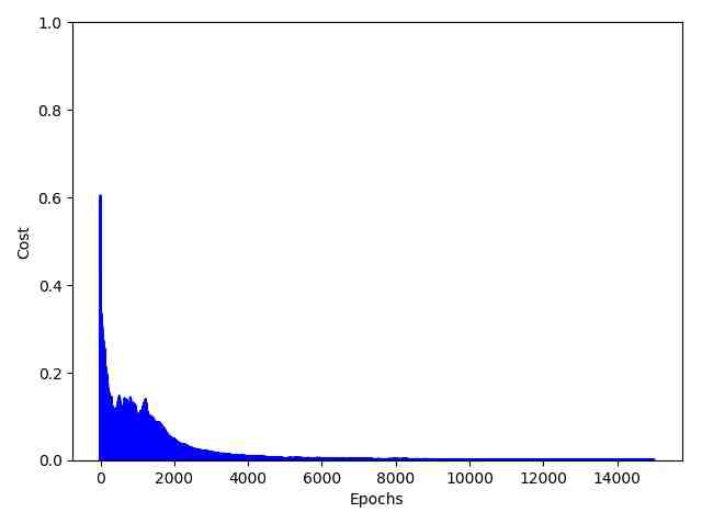

Finally we can see the hidden weights obtained and the output weights of the connections, as these values will be the ones we will use in the final network on our AdaCore code:

########## WE GENERATE THE GPS CODE
def to_str(name, W):
    s = str(W.tolist()).replace('[', '{').replace(']', '}')
    return 'float '+name+'['+str(W.shape[0])+']['+str(W.shape[1])+'] = ' + s + ';'

# We get the weights trained to be able to use them in the GPS code
pesos = nn.get_weights();

print('// Replace these lines in your arduino code:')
print('// float HiddenWeights ...')
print('// float OutputWeights ...')
print('// With trained weights.')
print('\n')
print(to_str('HiddenWeights', pesos[0]))
print(to_str('OutputWeights', pesos[1]))

Hidden weights and output weights of neural network

I repeat it, I modified these codes and ran them with Python and you can get in the download section. Now we are going to implement these coefficients in our AdaCore code.

GPS PROJECT

(Timing: 8 hrs.)

GNAT Programming Studio (GPS) is a free multi-language integrated development environment (IDE) by AdaCore. GPS uses compilers from the GNU Compiler Collection, taking its name from GNAT, the GNU compiler for the Ada programming language. Released under the GNU General Public License, GPS is free software. The download link is as follows: https://www.adacore.com/download

In my opinion, this is a powerful software with mathematical tools that allow us to develop high-precision projects as I explain below. First step, we have to download the next library: https://github.com/AdaCore/Ada_Drivers_Library

I'm the author of the following code, and to develop this GPS project, I used the following two examples: demo_gpio_direct_leds, and demo_adc_polling.

How does it work?

To start my project I have used the sample code: demo_adc_gpio_polling.adb; in my project I'm going to measure the analog signal generated by the LDR sensor through the analog port PA5, we will have 4095 values with its 12-bit CAD.

Converter     : Analog_To_Digital_Converter renames ADC_1;
Input_Channel : constant Analog_Input_Channel := 5;
Input         : constant GPIO_Point := PA5;

By default, this code has already configured and initialized the digital output ports of the green and red LEDS, ie PG13 and PG14. I have only added ports PD12 and PD13.

LED1       : GPIO_Point renames PG13; -- GREEN LED
LED2       : GPIO_Point renames PG14; -- RED LED
LED3       : GPIO_Point renames PD12;
LED4       : GPIO_Point renames PD13;

After the digital and analog ports have been configured, in the declaration of variables, I've loaded the weights of the neural network calculated in the previous section:

-------------------------------------------
--- NEURONAL NETWORKS' WEIGHTS
-------------------------------------------
HiddenWeights_1_1 := -0.8330212122953609;
HiddenWeights_1_2 := 1.0912649297996564;
HiddenWeights_1_3 := -0.6179969826549335;
HiddenWeights_1_4 := -1.0762413280914194;
HiddenWeights_2_1 := -0.7221015071612642;
HiddenWeights_2_2 := -0.3040531641938827;
HiddenWeights_2_3 := 1.424273154914373;
HiddenWeights_2_4 := 0.5226012446435597;
HiddenWeights_3_1 := -1.3873042452980089;
HiddenWeights_3_2 := 0.8796185107005765;
HiddenWeights_3_3 := 0.6115239126364166;
HiddenWeights_3_4 := -0.6941384010920131;
OutputWeights_1_1 := 0.4890791000431967;
OutputWeights_1_2 := -1.2072393706400335;
OutputWeights_1_3 := -1.1170823069750404;
OutputWeights_1_4 := 0.08254392928517773;
OutputWeights_2_1 := 1.2585395954445326;
OutputWeights_2_2 := 0.7259701403757809;
OutputWeights_2_3 := 0.05232196665284013;
OutputWeights_2_4 := 0.5379573853597585;
OutputWeights_3_1 := 1.3028834913318572;
OutputWeights_3_2 := -1.3073304956402805;
OutputWeights_3_3 := 0.1681659447995217;
OutputWeights_3_4 := -0.016766185238717802;
OutputWeights_4_1 := -0.38086087439361543;
OutputWeights_4_2 := 0.8415209522385925;
OutputWeights_4_3 := -1.527573567687556;
OutputWeights_4_4 := 0.476559350936026;

Once the program starts working, we calculate and load the input values, using the variables 'eval' and 'lux':

----------------------------------------------
-- CHARGE INPUT VALUES...
----------------------------------------------
if light_Current >= light_Before then -- If light_Current is greater than or equal to, move forward
   eval := 1.0;
else -- else, it turns counterclockwise
   eval := -1.0;
end if;
if light_Current <= 3750 then -- If light_Current is less than, move forward or turn to the left
   lux := 1.0;
else -- else, "Stop"
   lux := -1.0;
end if;
---------

I experimentally calibrated the lux value of 3750 with several models of LDR sensors... with this value, I found a satisfactory response to position the robot close to the light source and without impacting the lamp or losing it in its movement.

We multiply the input matrix by the matrix of the hidden weights, and to each accumulated result we calculate the hyperbolic tangent to obtain values between 1 and -1:

----------------------------------------------
-- Input * HiddenWeights
-- We use the Tanh to get values between 1 and -1
----------------------------------------------
Hidden_Layer_1_1 := Tanh(1.0*HiddenWeights_1_1 + eval*HiddenWeights_2_1 + lux*HiddenWeights_3_1);
Hidden_Layer_1_2 := Tanh(1.0*HiddenWeights_1_2 + eval*HiddenWeights_2_2 + lux*HiddenWeights_3_2);
Hidden_Layer_1_3 := Tanh(1.0*HiddenWeights_1_3 + eval*HiddenWeights_2_3 + lux*HiddenWeights_3_3);
Hidden_Layer_1_4 := Tanh(1.0*HiddenWeights_1_4 + eval*HiddenWeights_2_4 + lux*HiddenWeights_3_4);

Again we multiply the matrix of the hidden weights by the matrix of the output weights and to each accumulated result we also calculate the hyperbolic tangent.

----------------------------------------------
-- Hidden_Layers * OutputWeights
-- We use the Tanh to get values between 1 and -1
----------------------------------------------
Output_Layer_1_1 := Tanh(Hidden_Layer_1_1*OutputWeights_1_1 + Hidden_Layer_1_2*OutputWeights_2_1 + Hidden_Layer_1_3*OutputWeights_3_1 + Hidden_Layer_1_4*OutputWeights_4_1);
Output_Layer_1_2 := Tanh(Hidden_Layer_1_1*OutputWeights_1_2 + Hidden_Layer_1_2*OutputWeights_2_2 + Hidden_Layer_1_3*OutputWeights_3_2 + Hidden_Layer_1_4*OutputWeights_4_2);
Output_Layer_1_3 := Tanh(Hidden_Layer_1_1*OutputWeights_1_3 + Hidden_Layer_1_2*OutputWeights_2_3 + Hidden_Layer_1_3*OutputWeights_3_3 + Hidden_Layer_1_4*OutputWeights_4_3);
Output_Layer_1_4 := Tanh(Hidden_Layer_1_1*OutputWeights_1_4 + Hidden_Layer_1_2*OutputWeights_2_4 + Hidden_Layer_1_3*OutputWeights_3_4 + Hidden_Layer_1_4*OutputWeights_4_4);

For each value of the output matrix we calculate the absolute value to handle positive values and round the result:

----------------------------------------------
-- We charge absolute and integer values at the outputs
----------------------------------------------
Output_1 := Integer (abs (Output_Layer_1_1));
Output_2 := Integer (abs (Output_Layer_1_2));
Output_3 := Integer (abs (Output_Layer_1_3));
Output_4 := Integer (abs (Output_Layer_1_4));

Finally we use these output values to activate and deactivate the digital output pins, which in turn feed the L298N driver (IN1, IN2, IN3 and IN4). This process is repeated every 100 milliseconds.

----------------------------------------------
-- Activate the outputs according to the calculations of the neural network
----------------------------------------------
if Output_1 = 1 then
   LED1.Set;
else
   LED1.Clear;
end if;
if Output_2 = 1 then
   LED2.Set;
else
   LED2.Clear;
end if;
if Output_3 = 1 then
   LED3.Set;
else
   LED3.Clear;
end if;
if Output_4 = 1 then
   LED4.Set;
else
   LED4.Clear;
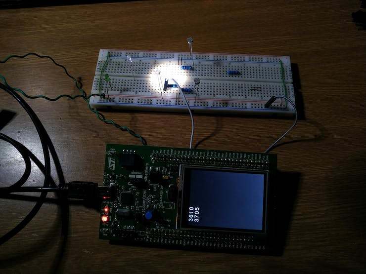
end if;

We can see the output status of these values on our LCD screen:

----------------------------------------------
-- Print the outputs of the neural network
----------------------------------------------
Print (0, 25, Output_1'Img);
Print (0, 50, Output_2'Img);
Print (0, 75, Output_3'Img);
Print (0, 100, Output_4'Img);

You must successfully compile and flash the code on your STM32F429I board. You can get the complete code in the download section.

Note: The code works well on the STM32F429I board, when it's powered by the PC. However, when the board is powered independently, the code doesn't run and the screen turns white. To correct this error you must update the firmware of your board... How? Simply download and update the firmware with the "STM32 ST-LINK Utility" application that you can download at: https://www.st.com/en/development-tools/stsw-link004.html

ASSEMBLING THE CHASSIS

(Timing: 4 hrs.)

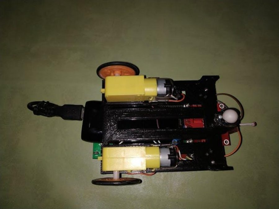
The two pieces that I printed with a 3D printer are the following: the Chassis is where we are going to adjust the two gear-motors, the L298N driver, the battery, and the LDR sensor module.

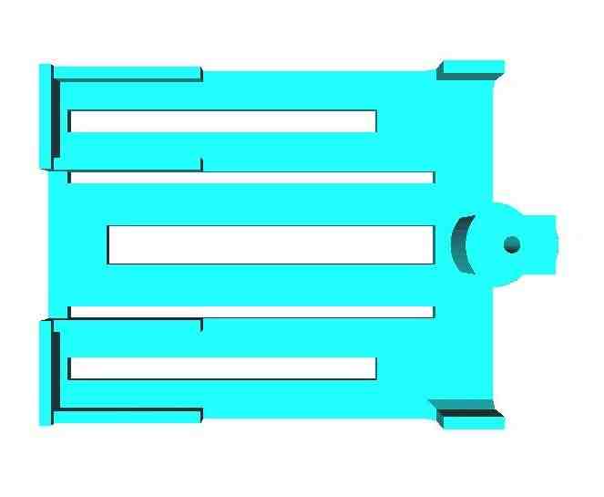
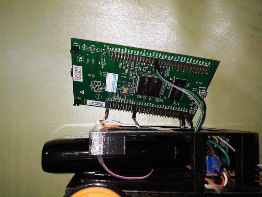
You can download the STL files in the downloads section. The upper part of the chassis is where we're going to adjust the STM32F429I board.

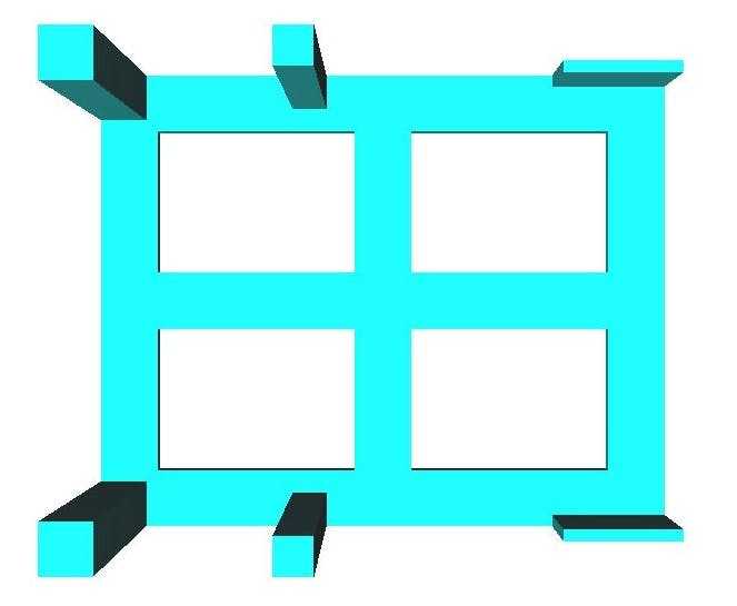
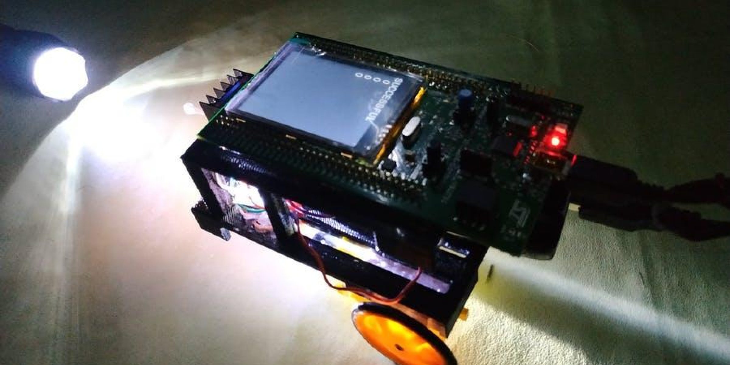
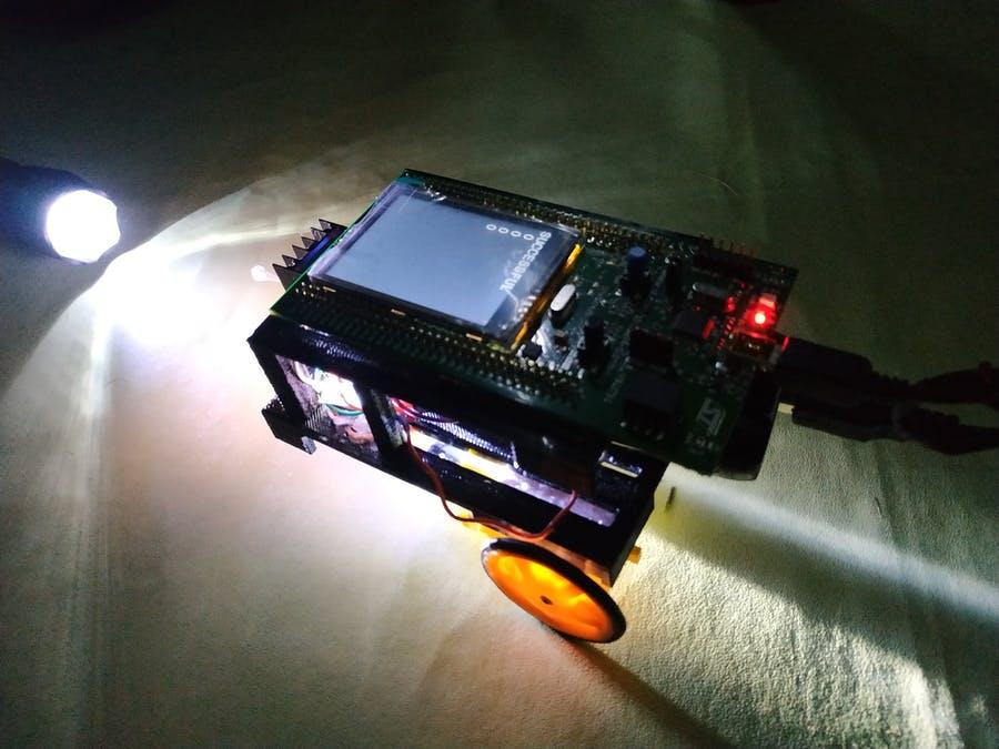
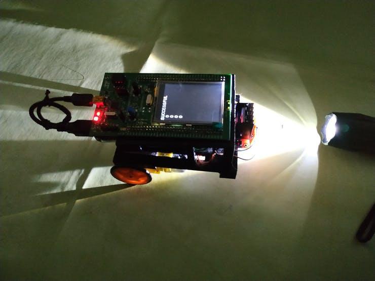
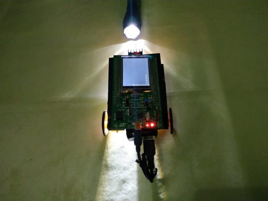
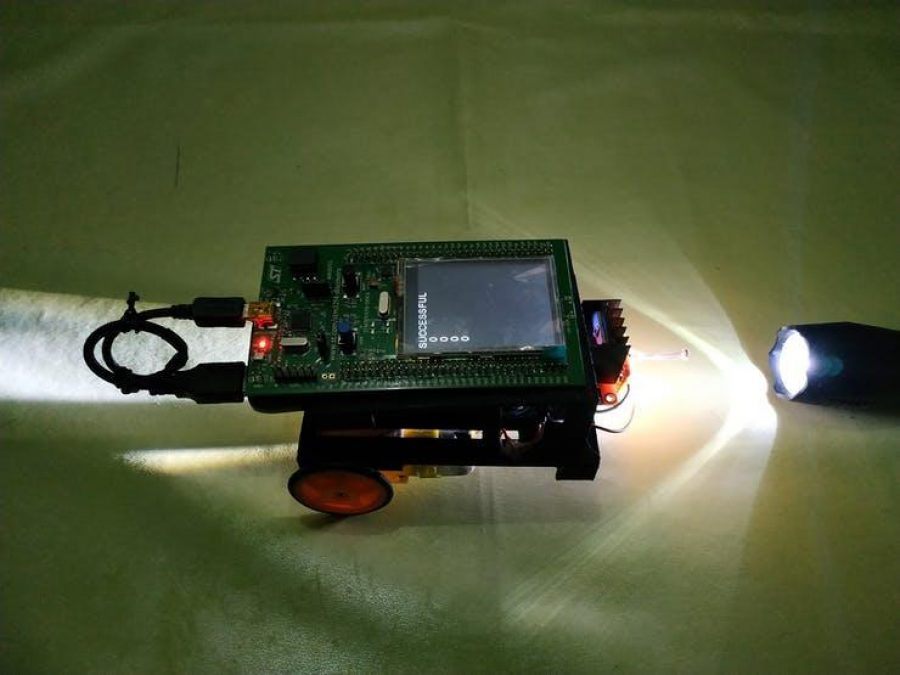
In figures below we can see several views of the assembly of our autonomous robot.

TEST

(Timing: 2 hrs.)

Below you can see a demonstration of how this prototype works.

CONCLUSION

In this project I learned and confirmed some theoretical concepts, and I'm contributing with an application of neural networks to the Adacore contest, and with an autonomous robot that showed us its effectiveness in developing its task. I didn't have to program all the situations or combinations that the robot would possibly face, and only 3 bits of information in the inputs were enough. This leads me to deduce that it's possible to add more bits of information to develop more complex tasks. The robot did find its target and also stopped when was necessary. I also demonstrated this smart device can be guided with a moving light, and that GPS libraries can make precision mathematical calculations with real-life problems. I recommend you do this kind of thing very carefully and verify every step.

Access the project schematics here.
Access the project code here.

Posted in

AdaCore Blog